Regression Notes - 1
This is the first notebook covering regression topics. It starts with basic estimation and diagnostics. This example uses a dataset I’m familiar with throu...
This is the first notebook covering regression topics. It starts with basic estimation and diagnostics. This example uses a dataset I’m familiar with through work experience, but it isn’t ideal for demonstrating more advanced topics.
The sample data I’m using for this is 3_3_Solar_Y2019.xlsx from form EIA-860, available here. The data contains generator-level solar energy data reported by utilities to the Energy Information Administration for calendar year 2019. For reasons that will shortly become clear, I am only interested in photovoltaic (PV) generators.
With respect to PV generators, this is a proxy for the size of the installation (bear in mind that a utility-owned PV generator as reported in the data often consists of multiple panels in a “solar farm”, but the panels in an installation should all have the same tilt). I’ll be regressing this capacity data on the panel tilt angle to see if there is any relationship while also controlling for a few other factors that could also affect installation capacity.
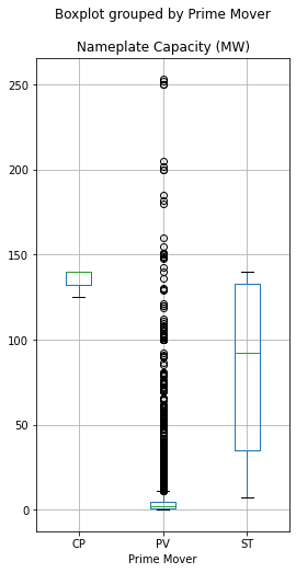
First, I’ll import the data and do some basic visualizations on generation capacity (the amount of power in megawatts that can be output by the generator) and compare it to that of thermal solar installations.
#import libraries and import data as dataframe
import pandas as pd
import matplotlib.pyplot as plt
import numpy as np
data = pd.read_excel (r'C:\Users\garre\Documents\Python Scripts\datasets\EIA-860\3_3_Solar_Y2019.xlsx', sheet_name = 'Operable', header=1)
data.boxplot(column = 'Nameplate Capacity (MW)', by = 'Prime Mover', figsize = (4,8) )
<AxesSubplot:title={'center':'Nameplate Capacity (MW)'}, xlabel='Prime Mover'>
groupedbypm = data.groupby(by = data['Prime Mover']).sum()
plt.pie(x = groupedbypm['Nameplate Capacity (MW)'], labels = groupedbypm.index )
([<matplotlib.patches.Wedge at 0x1ee05b98b80>,
  <matplotlib.patches.Wedge at 0x1ee05b9e0a0>,
  <matplotlib.patches.Wedge at 0x1ee05b9e520>],
 [Text(1.099376518408859, 0.03703067338323363, 'CP'),
  Text(-1.096464773848027, 0.08811923575698509, 'PV'),
  Text(1.0928768186678455, -0.12498103543517913, 'ST')])
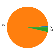
While they tend to be much larger than photovoltaic (PV) generators, solar thermal plants (CP and ST) are so few in number that they comprise only a small fraction of utility-owned solar generation capacity.
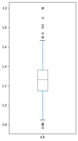
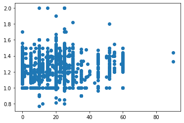
I’m interested in the relationship between PV panel tilt angle and the generator’s inverter loading ratio (the ratio of DC capacity to AC (nameplate) capacity).
First, I need to do some cleaning. I want to create a dataframe that only contains PV solar installations whose tilt angle was reported. I also need to refactor the tilt angle variable from object to float. Finally, I need to create a variable for the ILR.
There are some datapoints with unrealistically high ILR values. These are assumed to be due to reporting errors. Conservatively, we will drop observations with ILR values higher than two.
#create dataframe limited to photovoltaic generators whose tilt angle was reported
pvdata = data[(data['Prime Mover'] == 'PV') & (data['Tilt Angle']!=" ")].copy()
pvdata['Tilt Angle'] = pd.to_numeric(pvdata['Tilt Angle'])
#calculate Inverter Loading Ratio
pvdata['ILR'] = pvdata['DC Net Capacity (MW)']/pvdata['Nameplate Capacity (MW)']
pvdata['ILR'] = pd.to_numeric(pvdata['ILR'])
pvdata = pvdata.loc[pvdata['ILR']<=2]
pvdata['ILR'].plot.box(figsize = (4,8) )
<AxesSubplot:>
#scatter plot
plt.plot(pvdata['Tilt Angle'], pvdata['ILR'], 'o')
[<matplotlib.lines.Line2D at 0x1ee0874fa60>]
#obtain pearson correlation coefficient
from scipy.stats import pearsonr
pearsonr(pvdata['Tilt Angle'], pvdata['ILR'])
$\displaystyle \left( 0.08111342090515408, \ 2.274360325748276e-06\right)$
pearsonr(pvdata['Tilt Angle'], pvdata['Operating Year'])
$\displaystyle \left( 0.17748663027514733, \ 2.23648978601648e-25\right)$
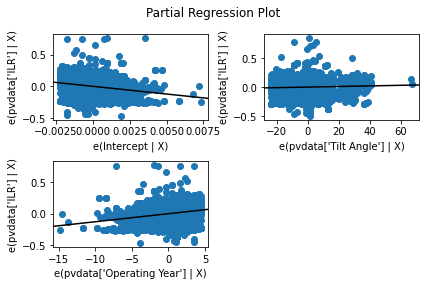
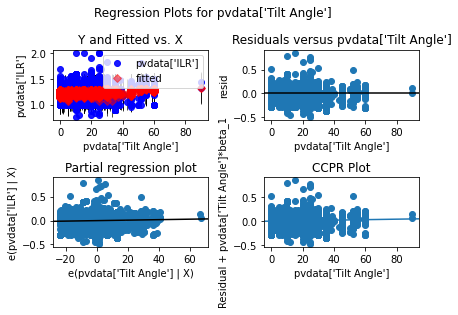
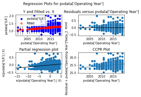
The first value in the tuple returned by the function is the coefficient. The second value is a two-tailed p-value. The variables don’t appear to be strongly correlated. Controlling for installation age might reveal a relationship, so let’s continue anyway. Let’s regress ILR on tilt angle, the year it was built.
import statsmodels.formula.api as sm
import statsmodels.api as sma
model = sm.ols(formula = "pvdata['ILR']~pvdata['Tilt Angle']+pvdata['Operating Year']", data = pvdata).fit(cov_type='HC1')
print(str(model.summary()))
                            OLS Regression Results
==============================================================================
Dep. Variable:          pvdata['ILR']   R-squared:                       0.055
Model:                            OLS   Adj. R-squared:                  0.054
Method:                 Least Squares   F-statistic:                     93.10
Date:                Thu, 05 Nov 2020   Prob (F-statistic):           4.35e-40
Time:                        17:40:04   Log-Likelihood:                 1566.2
No. Observations:                3388   AIC:                            -3126.
Df Residuals:                    3385   BIC:                            -3108.
Df Model:                           2
Covariance Type:                  HC1
============================================================================================
                               coef    std err          z      P>|z|      [0.025      0.975]
--------------------------------------------------------------------------------------------
Intercept                  -24.2847      2.010    -12.079      0.000     -28.225     -20.344
pvdata['Tilt Angle']         0.0005      0.000      2.618      0.009       0.000       0.001
pvdata['Operating Year']     0.0127      0.001     12.687      0.000       0.011       0.015
==============================================================================
Omnibus:                       51.091   Durbin-Watson:                   1.203
Prob(Omnibus):                  0.000   Jarque-Bera (JB):               79.362
Skew:                          -0.145   Prob(JB):                     5.84e-18
Kurtosis:                       3.692   Cond. No.                     1.50e+06
==============================================================================

Notes:
[1] Standard Errors are heteroscedasticity robust (HC1)
[2] The condition number is large, 1.5e+06. This might indicate that there are
strong multicollinearity or other numerical problems.
fitted = pd.DataFrame(model.fittedvalues, columns = ['Fitted'])
resid = pd.DataFrame(model.resid, columns = ['Resid'])
pvdata['yhat'] = fitted['Fitted']
pvdata['resid'] = resid['Resid']
pvdata.to_excel(r'C:\Users\garre\Documents\Python Scripts\datasets\EIA-860\post_reg_data.xlsx')
from statsmodels.stats.stattools import jarque_bera
from sympy import *
init_printing(use_unicode=True)
name = ['Jarque-Bera', 'Chi^2 two-tail prob.', 'Skew', 'Kurtosis']
normaltest = jarque_bera(model.resid)
x = (name, normaltest)
for line in x:
    print(*line)
Jarque-Bera Chi^2 two-tail prob. Skew Kurtosis
79.36218170079768 5.844148028089456e-18 -0.1446461440730232 3.6917353539381383
Jarque-Bera test results are reassuring, with skewness extremely close to 0, and kurtosis not far off from 3.
sma.graphics.plot_partregress_grid(model).tight_layout(pad=1.0)
sma.graphics.plot_regress_exog(model,"pvdata['Tilt Angle']" ).tight_layout(pad=1.0)
sma.graphics.plot_regress_exog(model,"pvdata['Operating Year']" ).tight_layout(pad=1.0)
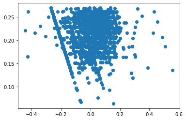
plt.plot(model.fittedvalues,model.resid, 'o')
[<matplotlib.lines.Line2D at 0x1ee0db36a00>]
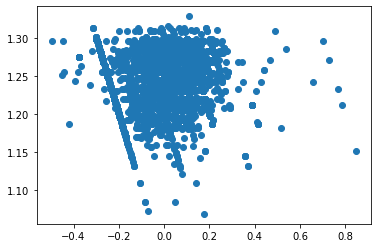
This is bizarre: A subset of the residuals form a perfect line.
plt.plot(model.fittedvalues[model.resid<0], model.resid[model.resid<0], 'o')
[<matplotlib.lines.Line2D at 0x1ee091bc580>]
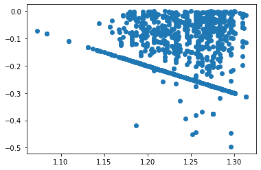
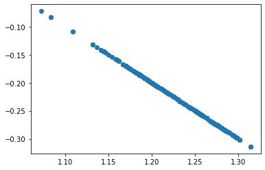
Further analysis of the data shows that these residuals correspond to an ILR value of 1:
plt.plot(pvdata['yhat'][pvdata['ILR']==1], pvdata['resid'][pvdata['ILR']==1], 'o')
[<matplotlib.lines.Line2D at 0x1ee05b68ee0>]
pvdata['Tilt Angle log'] = np.log(pvdata['Tilt Angle']+1)
pvdata['ILR log'] = np.log(pvdata['ILR'])
linearlogmodel = sm.ols(formula = "pvdata['ILR']~pvdata['Tilt Angle log']+pvdata['Operating Year']+pvdata['Crystalline Silicon?']", data = pvdata).fit()
loglinearmodel = sm.ols(formula = "pvdata['ILR log']~pvdata['Tilt Angle']+pvdata['Operating Year']+pvdata['Crystalline Silicon?']", data = pvdata).fit()
loglogmodel =  sm.ols(formula = "pvdata['ILR log']~pvdata['Tilt Angle log']+pvdata['Operating Year']+pvdata['Crystalline Silicon?']", data = pvdata).fit()
plt.plot(loglinearmodel.resid, loglinearmodel.fittedvalues,  'o')
plt.show()
plt.plot(linearlogmodel.resid, linearlogmodel.fittedvalues,  'o')
plt.show()
plt.plot(loglogmodel.resid, loglogmodel.fittedvalues,  'o')
plt.show()
This is the first notebook covering regression topics. It starts with basic estimation and diagnostics. This example uses a dataset I’m familiar with throu...
Now things are getting fun: We’re moving on to section 3, on conditional probability and independence! If you’re on mobile, you can view the lesson here: Pr...
This is the coding supplement to theory lesson 1-2-6. If you’re on mobile, view this lesson here: Lesson R-1-2-6: Counting. You can also download the code ...
Short final lesson on calculating probabilities by counting. If you’re on mobile, you can view the lesson here: Presentation 1-2-7: Finishing Up
And now for the thrilling conclusion to our two-part lesson on counting! If you’re on mobile, you can view the lesson here: Presentation 1-2-6 Learning to Co...
Think you know how to count? Well, think again! It’s time we covered the Fundamental Theorem of Counting! This two-part lesson will be followed up by a cod...
We’re pretty close to finishing the material from subsection 1.2.2: The Calculus of Probabilities. Enjoy this short lesson on Bonferroni’s Inequality. Next...
Pretty soon we’re gonna need to write some code. Luckily, I’m here to teach you how to do it! We’re gonna start by installing R and RStudio. Then, we’ll g...
Now it’s getting serious. We’ve established the axioms of probability, but there is so much more to be done with them! Some of it, sadly, gets a little inv...
Now we’re getting to the good stuff! We’re not only taking a deeper dive into the axioms of probability, we’re also proving that a (relatively) simple funct...
We’re ready to start working toward an axiomatic definition of probability. First, however, we take a rather painful detour through the realm of Borel field...
This lesson rounds out our primer on set theory by introducing operators that allow us to take the union or intersection of many (or even infinitely many) se...
This lesson explores event operations, specifically unions, intersections, and complementation, as well as the properties of these operations with detailed v...
This lesson begins our journey with the introduction of the sample space, and the events therein. If you’re on mobile, you can view the lesson here: Present...